Rotating reference frame

Classical mechanics
$\mathbf{F} = m \mathbf{a}$ Newton's Second Law
History of classical mechanics · Timeline of classical mechanics
Branches Statics · Dynamics / Kinetics · Kinematics · Applied mechanics · Celestial mechanics · Continuum mechanics · Statistical mechanics
Formulations Newtonian mechanics (Vectorial mechanics) Analytical mechanics: Lagrangian mechanics Hamiltonian mechanics
Fundamental concepts Space · Time · Velocity · Speed · Mass · Acceleration · Gravity · Force · Impulse · Torque / Moment / Couple · Momentum · Angular momentum · Inertia · Moment of inertia · Reference frame · Energy · Kinetic energy · Potential energy · Mechanical work · Virtual work · D'Alembert's principle
Core topics Rigid body · Rigid body dynamics · Euler's equations (rigid body dynamics) · Motion · Newton's laws of motion · Newton's law of universal gravitation · Euler's laws of motion · Equations of motion · Inertial frame of reference · Non-inertial reference frame · Rotating reference frame · Fictitious force · Linear motion · Mechanics of planar particle motion · Displacement (vector) · Relative velocity · Friction · Simple harmonic motion · Harmonic oscillator · Vibration · Damping · Damping ratio · Rotational motion · Circular motion · Uniform circular motion · Non-uniform circular motion · Centripetal force · Centrifugal force · Centrifugal force (rotating reference frame) · Reactive centrifugal force · Coriolis force · Pendulum · Rotational speed · Angular acceleration · Angular velocity · Angular frequency · Angular displacement
Scientists Galileo Galilei · Isaac Newton · Jeremiah Horrocks · Leonhard Euler · Jean le Rond d'Alembert · Alexis Clairaut · Joseph Louis Lagrange · Pierre-Simon Laplace · William Rowan Hamilton · Siméon-Denis Poisson

A rotating frame of reference is a special case of a non-inertial reference frame that is rotating relative to an inertial reference frame. An everyday example of a rotating reference frame is the surface of the Earth. (This article considers only frames rotating about a fixed axis. For more general rotations, see Euler angles.)

1 Fictitious forces
2 Relating rotating frames to stationary frames
3 Centrifugal force
4 Coriolis effect
5 Euler force
6 References and notes
7 See also
8 External links

Fictitious forces

Main article: Fictitious forces

All non-inertial reference frames exhibit fictitious forces. Rotating reference frames are characterized by three fictitious forces^[1]

the centrifugal force
the Coriolis force

and, for non-uniformly rotating reference frames,

the Euler force.

Scientists living in a rotating box can measure the speed and direction of their rotation by measuring these fictitious forces. For example, Léon Foucault was able to show the Coriolis force that results from the Earth's rotation using the Foucault pendulum. If the Earth were to rotate a thousandfold faster (making each day only ~86 seconds long), these fictitious forces could be felt as easily by humans, as they are when on a spinning carousel.

Relating rotating frames to stationary frames

The following is a derivation of the formulas for accelerations as well as fictitious forces in a rotating frame. It begins with the relation between coordinates of the position of a particle in a rotating frame and the coordinates in an inertial (stationary) frame. Then, by taking time derivatives, formulas are derived that relate the velocity of the particle as seen in the two frames, and the acceleration relative to each frame. Using these accelerations a comparison of Newton's second law as formulated in the frames identifies the fictitious forces.

Relation between positions in the two frames

To derive these fictitious forces, it's helpful to be able to convert between the coordinates $\left( x',y',z' \right)$ of the rotating reference frame and the coordinates $\left( x, y, z \right)$ of an inertial reference frame with the same origin. If the rotation is about the $z$ axis with an angular velocity $\Omega$ and the two reference frames coincide at time $t=0$ , the transformation from rotating coordinates to inertial coordinates can be written

$x = x'\cos\left(\Omega t\right) - y'\sin\left(\Omega t\right)$

$y = x'\sin\left(\Omega t\right) %2B y'\cos\left(\Omega t\right)$

whereas the reverse transformation is

$x' = x\cos\left(-\Omega t\right) - y\sin\left( -\Omega t \right)$

$y' = x\sin\left( -\Omega t \right) %2B y\cos\left( -\Omega t \right)$

This result can be obtained from a rotation matrix.

Introduce the unit vectors $\hat{\boldsymbol{\imath}},\ \hat{\boldsymbol{\jmath}},\ \hat{\boldsymbol{k}}$ representing standard unit basis vectors in the rotating frame. The time-derivatives of these unit vectors are found next. Suppose the frames are aligned at t = 0 and the z-axis is the axis of rotation. Then for a counterclockwise rotation through angle Ωt:

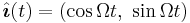
$\hat{\boldsymbol{\imath}}(t) = (\cos\Omega t,\ \sin \Omega t )$

where the (x, y) components are expressed in the stationary frame. Likewise,

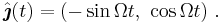
$\hat{\boldsymbol{\jmath}}(t) = (-\sin \Omega t,\ \cos \Omega t ) \ .$

Thus the time derivative of these vectors, which rotate without changing magnitude, is

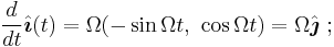
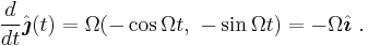
$\frac{d}{dt}\hat{\boldsymbol{\imath}}(t) = \Omega (-\sin \Omega t, \ \cos \Omega t)= \Omega \hat{\boldsymbol{\jmath}} \�;$

$\frac{d}{dt}\hat{\boldsymbol{\jmath}}(t) = \Omega (-\cos \Omega t, \ -\sin \Omega t)= - \Omega \hat{\boldsymbol{\imath}} \ .$

This result is the same as found using a vector cross product with the rotation vector $\boldsymbol{\Omega}$ pointed along the z-axis of rotation $\boldsymbol{\Omega}=(0,\ 0,\ \Omega)$ , namely,

$\frac{d}{dt}\hat{\boldsymbol{u}} = \boldsymbol{\Omega \times}\hat {\boldsymbol{ u}} \ ,$

where $\hat {\boldsymbol{ u}}$ is either $\hat{\boldsymbol{\imath}}$ or $\hat{\boldsymbol{\jmath}}$ .

Time derivatives in the two frames

Introduce the unit vectors $\hat{\boldsymbol{\imath}},\ \hat{\boldsymbol{\jmath}},\ \hat{\boldsymbol{k}}$ representing standard unit basis vectors in the rotating frame. As they rotate they will remain normalized. If we let them rotate at the speed of $\Omega$ about an axis $\boldsymbol {\Omega}$ then each unit vector $\hat{\boldsymbol{u}}$ of the rotating coordinate system abides by the following equation:

$\frac{d}{dt}\hat{\boldsymbol{u}}=\boldsymbol{\Omega \times \hat{u}} \ .$

Then if we have a vector function $\boldsymbol{f}$ ,

$\boldsymbol{f}(t)=f_x(t) \hat{\boldsymbol{\imath}}%2Bf_y(t) \hat{\boldsymbol{\jmath}}%2Bf_z(t) \hat{\boldsymbol{k}}\ ,$

and we want to examine its first dervative we have (using the product rule of differentiation):^[2]^[3]

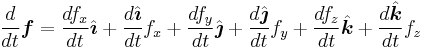
$\frac{d}{dt}\boldsymbol{f}=\frac{df_x}{dt}\hat{\boldsymbol{\imath}}%2B\frac{d\hat{\boldsymbol{\imath}}}{dt}f_x%2B\frac{df_y}{dt}\hat{\boldsymbol{\jmath}}%2B\frac{d\hat{\boldsymbol{\jmath}}}{dt}f_y%2B\frac{df_z}{dt}\hat{\boldsymbol{k}}%2B\frac{d\hat{\boldsymbol{k}}}{dt}f_z$

$=\frac{df_x}{dt}\hat{\boldsymbol{\imath}}%2B\frac{df_y}{dt}\hat{\boldsymbol{\jmath}}%2B\frac{df_z}{dt}\hat{\boldsymbol{k}}%2B[\boldsymbol{\Omega \times} (f_x \hat{\boldsymbol{\imath}} %2B f_y \hat{\boldsymbol{\jmath}}%2Bf_z \hat{\boldsymbol{k}})]$

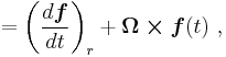
$= \left( \frac{d\boldsymbol{f}}{dt}\right)_r%2B\boldsymbol{\Omega \times f}(t)\ ,$

where $\left( \frac{d\boldsymbol{f}}{dt}\right)_r$ is the rate of change of $\boldsymbol{f}$ as observed in the rotating coordinate system. As a shorthand the differentiation is expressed as:

$\frac{d}{dt}\boldsymbol{f} =\left[ \left(\frac{d}{dt}\right)_r %2B \boldsymbol{\Omega \times} \right] \boldsymbol{f} \ .$

This result is also known as the Transport Theorem in analytical dynamics, and is also sometimes referred to as the Basic Kinematic Equation.^[4]

Relation between velocities in the two frames

A velocity of an object is the time-derivative of the object's position, or

$\mathbf{v} \ \stackrel{\mathrm{def}}{=}\ \frac{d\mathbf{r}}{dt}$

The time derivative of a position $\boldsymbol{r}(t)$ in a rotating reference frame has two components, one from the explicit time dependence due to motion of the particle itself, and another from the frame's own rotation. Applying the result of the previous subsection to the displacement $\boldsymbol{r}(t)$ , the velocities in the two reference frames are related by the equation

$\mathbf{v_i} \ \stackrel{\mathrm{def}}{=}\ \frac{d\mathbf{r}}{dt} = \left( \frac{d\mathbf{r}}{dt} \right)_{\mathrm{r}} %2B \boldsymbol\Omega \times \mathbf{r} = \mathbf{v}_{\mathrm{r}} %2B \boldsymbol\Omega \times \mathbf{r} \ ,$

where subscript i means the inertial frame of reference, and r means the rotating frame of reference.

Relation between accelerations in the two frames

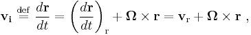
Acceleration is the second time derivative of position, or the first time derivative of velocity

$\mathbf{a}_{\mathrm{i}} \ \stackrel{\mathrm{def}}{=}\ \left( \frac{d^{2}\mathbf{r}}{dt^{2}}\right)_{\mathrm{i}} = \left( \frac{d\mathbf{v}}{dt} \right)_{\mathrm{i}} = \left[ \left( \frac{d}{dt} \right)_{\mathrm{r}} %2B \boldsymbol\Omega \times \right] \left[ \left( \frac{d\mathbf{r}}{dt} \right)_{\mathrm{r}} %2B \boldsymbol\Omega \times \mathbf{r} \right] \ ,$

where subscript i means the inertial frame of reference. Carrying out the differentiations and re-arranging some terms yields the acceleration in the rotating reference frame

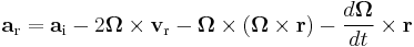
$\mathbf{a}_{\mathrm{r}} = \mathbf{a}_{\mathrm{i}} - 2 \boldsymbol\Omega \times \mathbf{v}_{\mathrm{r}} - \boldsymbol\Omega \times (\boldsymbol\Omega \times \mathbf{r}) - \frac{d\boldsymbol\Omega}{dt} \times \mathbf{r}$

where $\mathbf{a}_{\mathrm{r}} \ \stackrel{\mathrm{def}}{=}\ \left( \frac{d^{2}\mathbf{r}}{dt^{2}} \right)_{\mathrm{r}}$ is the apparent acceleration in the rotating reference frame, the term $-\boldsymbol\Omega \times (\boldsymbol\Omega \times \mathbf{r})$ represents centrifugal acceleration, and the term $-2 \boldsymbol\Omega \times \mathbf{v}_{\mathrm{r}}$ is the coriolis effect.

Newton's second law in the two frames

When the expression for acceleration is multiplied by the mass of the particle, the three extra terms on the right-hand side result in fictitious forces in the rotating reference frame, that is, apparent forces that result from being in a non-inertial reference frame, rather than from any physical interaction between bodies.

Using Newton's second law of motion $\mathbf{F}=m\mathbf{a}$ , we obtain:^[1]^[2]^[3]^[5]^[6]

the Coriolis force

$\mathbf{F}_{\mathrm{Coriolis}} = -2m \boldsymbol\Omega \times \mathbf{v}_{\mathrm{r}}$

the centrifugal force

$\mathbf{F}_{\mathrm{centrifugal}} = -m\boldsymbol\Omega \times (\boldsymbol\Omega \times \mathbf{r})$

and the Euler force

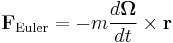
$\mathbf{F}_{\mathrm{Euler}} = -m\frac{d\boldsymbol\Omega}{dt} \times \mathbf{r}$

where $m$ is the mass of the object being acted upon by these fictitious forces. Notice that all three forces vanish when the frame is not rotating, that is, when $\boldsymbol{\Omega} = 0 \ .$

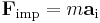
For completeness, the inertial acceleration $\mathbf{a}_{\mathrm{i}}$ due to impressed external forces $\mathbf{F}_{\mathrm{imp}}$ can be determined from the total physical force in the inertial (non-rotating) frame (for example, force from physical interactions such as electromagnetic forces) using Newton's second law in the inertial frame:

$\mathbf{F}_{\mathrm{imp}} = m \mathbf{a}_{\mathrm{i}}$

Newton's law in the rotating frame then becomes

$\mathbf{F_r} = \mathbf{F}_{\mathrm{imp}} %2B\mathbf{F}_{\mathrm{centrifugal}} %2B\mathbf{F}_{\mathrm{Coriolis}}%2B\mathbf{F}_{\mathrm{Euler}} = m\mathbf{a_r} \ .$

In other words, to handle the laws of motion in a rotating reference frame:^[6]^[7]^[8]

Treat the fictitious forces like real forces, and pretend you are in an inertial frame.

— Louis N. Hand, Janet D. Finch Analytical Mechanics, p. 267

Obviously, a rotating frame of reference is a case of a non-inertial frame. Thus the particle in addition to the real force is acted upon by a fictitious force...The particle will move according to Newton's second law of motion if the total force acting on it is taken as the sum of the real and fictitious forces.

— HS Hans & SP Pui: Mechanics; p. 341

This equation has exactly the form of Newton's second law, except that in addition to F, the sum of all forces identified in the inertial frame, there is an extra term on the right...This means we can continue to use Newton's second law in the noninertial frame provided we agree that in the noninertial frame we must add an extra force-like term, often called the inertial force.

— John R. Taylor: Classical Mechanics; p. 328

Centrifugal force

Main article: Centrifugal force (rotating reference frame)

In classical mechanics, centrifugal force is an outward force associated with rotation. Centrifugal force is one of several so-called pseudo-forces (also known as inertial forces), so named because, unlike real forces, they do not originate in interactions with other bodies situated in the environment of the particle upon which they act. Instead, centrifugal force originates in the rotation of the frame of reference within which observations are made.^[9]^[10]^[11]^[12]^[13]^[14]

Coriolis effect

Main article: Coriolis effect

The mathematical expression for the Coriolis force appeared in an 1835 paper by a French scientist Gaspard-Gustave Coriolis in connection with hydrodynamics, and also in the tidal equations of Pierre-Simon Laplace in 1778. Early in the 20th century, the term Coriolis force began to be used in connection with meteorology.

Perhaps the most commonly encountered rotating reference frame is the Earth. Moving objects on the surface of the Earth experience a Coriolis force, and appear to veer to the right in the northern hemisphere, and to the left in the southern. Movements of air in the atmosphere and water in the ocean are notable examples of this behavior: rather than flowing directly from areas of high pressure to low pressure, as they would on a non-rotating planet, winds and currents tend to flow to the right of this direction north of the equator, and to the left of this direction south of the equator. This effect is responsible for the rotation of large cyclones (see Coriolis effects in meteorology).

Euler force

Main article: Euler force

In classical mechanics, the Euler acceleration (named for Leonhard Euler), also known as azimuthal acceleration^[15] or transverse acceleration^[16] is an acceleration that appears when a non-uniformly rotating reference frame is used for analysis of motion and there is variation in the angular velocity of the reference frame's axis. This article is restricted to a frame of reference that rotates about a fixed axis.

The Euler force is a fictitious force on a body that is related to the Euler acceleration by F = m a , where a is the Euler acceleration and m is the mass of the body.^[17]^[18]

References and notes

^ ^a ^b Vladimir Igorević Arnolʹd (1989). Mathematical Methods of Classical Mechanics (2nd Edition ed.). Springer. p. 130. ISBN 978-0-387-96890-2. http://books.google.com/books?id=Pd8-s6rOt_cC&pg=PT149&dq=%22additional+terms+called+inertial+forces.+This+allows+us+to+detect+experimentally%22#PPT150,M1.
^ ^a ^b Cornelius Lanczos (1986). The Variational Principles of Mechanics (Reprint of Fourth Edition of 1970 ed.). Dover Publications. Chapter 4, §5. ISBN 0-486-65067-7. http://books.google.com/books?num=10&btnG=Google+Search.
^ ^a ^b John R Taylor (2005). Classical Mechanics. University Science Books. p. 342. ISBN 1-891389-22-X. http://books.google.com/books?id=P1kCtNr-pJsC&pg=PP1&dq=isbn=189138922X#PPA342,M1.
^ Corless, Martin. "Kinematics". Aeromechanics I Course Notes. Purdue University. p. 213. https://engineering.purdue.edu/AAE/Academics/Courses/aae203/2003/fall/aae203F03supp.pdf. Retrieved 18 July 2011.
^ LD Landau and LM Lifshitz (1976). Mechanics (Third Edition ed.). p. 128. ISBN 978-0-7506-2896-9. http://books.google.com/books?id=e-xASAehg1sC&pg=PA40&dq=isbn=9780750628969#PPA128,M1.
^ ^a ^b Louis N. Hand, Janet D. Finch (1998). Analytical Mechanics. Cambridge University Press. p. 267. ISBN 0521575729. http://books.google.com/books?id=1J2hzvX2Xh8C&pg=PA267&vq=fictitious+forces&dq=Hand+inauthor:Finch.
^ HS Hans & SP Pui (2003). Mechanics. Tata McGraw-Hill. p. 341. ISBN 0070473609. http://books.google.com/books?id=mgVW00YV3zAC&pg=PA341&dq=inertial+force+%22rotating+frame%22.
^ John R Taylor (2005). Classical Mechanics. University Science Books. p. 328. ISBN 1-891389-22-X. http://books.google.com/books?id=P1kCtNr-pJsC&pg=PP1&dq=isbn=189138922X#PPA328,M1.
^ Robert Resnick & David Halliday (1966). Physics. Wiley. p. 121. ISBN 0471345245. http://books.google.com/books?q=%22cannot+associate+them+with+any+particular+body+in+the+environment+of+the+particle%22+inauthor%3ADavid+inauthor%3AHalliday&btnG=Search+Books.
^ Jerrold E. Marsden, Tudor S. Ratiu (1999). Introduction to Mechanics and Symmetry: A Basic Exposition of Classical Mechanical Systems. Springer. p. 251. ISBN 038798643X. http://books.google.com/books?id=I2gH9ZIs-3AC&pg=PA251&vq=Euler+force&dq=isbn=038798643X.
^ John Robert Taylor (2005). Classical Mechanics. University Science Books. p. 343. ISBN 189138922X. http://books.google.com/books?id=P1kCtNr-pJsC&pg=PP1&dq=isbn=189138922X#PPA343,M1.
^ Stephen T. Thornton & Jerry B. Marion (2004). Classical Dynamics of Particles and Systems (5th ed.). Belmont CA: Brook/Cole. Chapter 10. ISBN 0534408966. http://worldcat.org/oclc/52806908&referer=brief_results.
^ David McNaughton. "Centrifugal and Coriolis Effects". http://dlmcn.com/circle.html. Retrieved 2008-05-18.
^ David P. Stern. "Frames of reference: The centrifugal force". http://www.phy6.org/stargaze/Lframes2.htm. Retrieved 2008-10-26.
^ David Morin (2008). Introduction to classical mechanics: with problems and solutions. Cambridge University Press. p. 469. ISBN 0521876222. http://books.google.com/books?id=Ni6CD7K2X4MC&pg=PA469&dq=acceleration+azimuthal+inauthor:Morin.
^ Grant R. Fowles and George L. Cassiday (1999). Analytical Mechanics, 6th ed.. Harcourt College Publishers. p. 178.
^ Richard H Battin (1999). An introduction to the mathematics and methods of astrodynamics. Reston, VA: American Institute of Aeronautics and Astronautics. p. 102. ISBN 1563473429. http://books.google.com/books?id=OjH7aVhiGdcC&pg=PA102&vq=Euler&dq=%22Euler+acceleration%22.
^ Jerrold E. Marsden, Tudor S. Ratiu (1999). Introduction to Mechanics and Symmetry: A Basic Exposition of Classical Mechanical Systems. Springer. p. 251. ISBN 038798643X. http://books.google.com/books?id=I2gH9ZIs-3AC&pg=PP1&dq=isbn:038798643X#PPA251,M1.

External links

Animation clip showing scenes as viewed from both an inertial frame and a rotating frame of reference, visualizing the Coriolis and centrifugal forces.